Lecture 3: Optimal Policy and Bellman Optimality Equation

1-Outline

In this lecture:

• Core concepts: optimal policy and optimal state value
• A fundamental tool: Bellman optimality equation (BOE)

2-Motivating examples

• Exercise: write out the Bellman equation and solve the state values (set $\gamma = 0.9$)

• Bellman equations:

$$v_\pi(s_1) = -1 + \gamma v_\pi(s_2),$$

$$v_\pi(s_2) = +1 + \gamma v_\pi(s_4),$$

$$v_\pi(s_3) = +1 + \gamma v_\pi(s_4),$$

$$v_\pi(s_4) = +1 + \gamma v_\pi(s_4).$$

• State values: $v_\pi(s_4) = v_\pi(s_3) = v_\pi(s_2) = 10, v_\pi(s_1) = 8$

• Exercise: calculate the action values of the five actions for $s_1$

• Action values:

$$q_\pi(s_1, a_1) = -1 + \gamma v_\pi(s_1) = 6.2,$$

$$q_\pi(s_1, a_2) = -1 + \gamma v_\pi(s_2) = 8,$$

$$q_\pi(s_1, \textcolor{orange}{a_3}) = 0 + \gamma v_\pi(s_3) = 9,$$

$$q_\pi(s_1, a_4) = -1 + \gamma v_\pi(s_1) = 6.2,$$

$$q_\pi(s_1, a_5) = 0 + \gamma v_\pi(s_1) = 7.2.$$

• Question: While the policy is not good, how can we improve it?
• Answer: We can improve the policy based on action values.

In particular, the current policy $\pi(a|s_1)$ is:

$$\pi(a|s_1) = \begin{cases} 1 & a = a_2 \\ 0 & a \neq a_2 \end{cases}$$

Observe the action values that we obtained just now:

$$q_\pi(s_1, a_1) = 6.2, \quad q_\pi(s_1, a_2) = 8, \quad q_\pi(s_1, a_3) = 9,$$

$$q_\pi(s_1, a_4) = 6.2, \quad q_\pi(s_1, a_5) = 7.2.$$

What if we select the greatest action value? Then, the new policy is

$$\pi_{new}(a|s_1) = \begin{cases} 1 & a = a_3 \\ 0 & a \neq a_3 \end{cases}$$

• Question: Why doing this can improve the policy?
• Intuition: Action values can be used to evaluate actions.
• Math: nontrivial and will be introduced in the this lecture.

3-Definition of optimal policy

The state value could be used to evaluate if a policy is good or not: if

$$v_{\pi_1}(s) \geq v_{\pi_2}(s) \quad \text{for all} \quad s \in \mathcal{S}$$

then $\pi_1$ is “better” than $\pi_2$.

• Definition: A policy $\pi^*$ is optimal if $v_{\pi^*}(s) \geq v_\pi(s)$ for all $s$ and for any other policy $\pi$.

The definition leads to many questions:

• Does the optimal policy exist?
• Is the optimal policy unique?
• Is the optimal policy stochastic or deterministic?
• How to obtain the optimal policy?
  To answer these questions, we study the Bellman optimality equation.

4-BOE: Introduction

• Bellman optimality equation (elementwise form):

$$v(s) = \max_\pi \sum_a \pi(a|s) \left(\sum_r p(r|s,a)r + \gamma \sum_{s'} p(s'|s,a)v(s')\right), \quad s \in \mathcal{S}$$

$$= \max_\pi \sum_a \pi(a|s)q(s,a), \quad s \in \mathcal{S}$$

• Remarks:

  • $p(r|s,a), p(s'|s,a), r, \gamma$ are known.
  • $v(s), v(s')$ are unknown and to be calculated.
  • Is $\pi(s)$ known or unknown?

• Bellman optimality equation (matrix-vector form):

$$v = \max_\pi (r_\pi + \gamma P_\pi v)$$

where the elements corresponding to $s$ or $s'$ are

$$[r_\pi]_s \triangleq \sum_a \pi(a|s) \sum_r p(r|s,a)r,$$

$$[P_\pi]_{s,s'} = p(s'|s) \triangleq \sum_a \pi(a|s) \sum_{s'} p(s'|s,a)$$

Here $\max_\pi$ is performed elementwise:

$$\max_\pi \begin{bmatrix} * \\ \vdots \\ * \end{bmatrix} = \begin{bmatrix} \max_{\pi(s_1)} * \\ \vdots \\ \max_{\pi(s_n)} * \end{bmatrix}$$

• Remarks:
  • BOE is tricky yet elegant!
  • Why elegant? It describes the optimal policy and optimal state value in an elegant way.
  • Why tricky? There is a maximization on the right-hand side, which may not be straightforward to see how to compute.
  • This lecture will answer all the following questions:
    • Algorithm: how to solve this equation?
    • Existence: does this equation have solutions?
    • Uniqueness: is the solution to this equation unique?
    • Optimality: how is it related to optimal policy?

5-BOE: Preliminaries

5.1-BOE: Maximization on the right-hand side

5.2-BOE: Rewrite as $\mathbb{v} = f(\mathbb{v})$

The BOE is $v = \max_\pi(r_\pi + \gamma P_\pi v)$. Let

$$f(v) := \max_\pi(r_\pi + \gamma P_\pi v)$$

Then, the Bellman optimality equation becomes

$$v = f(v)$$

where

$$[f(v)]_s = \max_\pi \sum_a \pi(a|s)q(s,a), \quad s \in \mathcal{S}$$

This equation looks very simple. How to solve it?

5.3-Contraction mapping theorem（压缩映射定理）

Some concepts:

• Fixed point: $x \in X$ is a fixed point of $f: X \rightarrow X$ if

$$f(x) = x$$

• Contraction mapping: $f: X \rightarrow X$ is a contraction mapping if

$$||f(x_1) - f(x_2)|| \leq \gamma ||x_1 - x_2||$$

where $\gamma \in (0, 1)$.

• Remarks:
  • $\gamma$ must be strictly less than 1 so that many limits such as $\gamma^{k} \rightarrow 0$ as $k \rightarrow \infty$ hold.
  • Here $|| \cdot ||$ is the norm of the vector space $X$.

Examples to demonstrate the concepts:

Above all, we can get the definition of Contraction Mapping Theorem:

6-BOE: Solution

6.1-Contraction property of BOE

Let’s come back to the Bellman optimality equation:

$$v = f(v) = \max_\pi(r_\pi + \gamma P_\pi v)$$

6.2-Solve the Bellman optimality equation

Applying the contraction mapping theorem gives the following results:

Importance:The algorithm in (1) is called the value iteration algorithm.

7-Optimality

7.1-Policy Optimality

Suppose $v^*$ is the solution to the Bellman optimality equation. It satisfies

$$v^* = \max_\pi(r_\pi + \gamma P_\pi v^*)$$

Suppose

$$\pi^* = \arg \max_\pi(r_\pi + \gamma P_\pi v^*)$$

Then

$$v^* = r_{\pi^*} + \gamma P_{\pi^*} v^*$$

Therefore, $\pi^*$ is a policy and $v^* = v_{\pi^*}$ is the corresponding state value.

Is $\pi^*$ the optimal policy? Is $v^*$ the greatest state value can be achieved?

Now we understand why we study the BOE. That is because it describes the optimal state value and optimal policy in an elegant way.

7.2-Optimal policy

What does an optimal policy $\pi^*$ look like?

$$\pi^*(s) = \arg \max_\pi \sum_a \pi(a|s) \underbrace{\left(\sum_r p(r|s,a)r + \gamma \sum_{s'} p(s'|s,a)v^*(s')\right)}_{q^*(s,a)}$$

8-Analyzing optimal policies

What factors determine the optimal state value and optimal policy?
It can be clearly seen from the BOE

$${v(s)} = {\max_\pi} \sum_a {\pi(a|s)} \left(\sum_r \textcolor{red}{p(r|s,a)}r + \textcolor{red}{\gamma} \sum_{s'} \textcolor{red}{p(s'|s,a)}{v(s')}\right)$$

that there are three factors:

• System model: ${p(s'|s,a)}$, ${p(r|s,a)}$
• Reward design: $r$
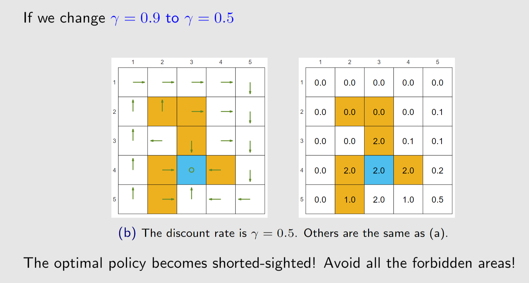
• Discount rate: ${\gamma}$

We next show how $r$ and ${\gamma}$ can affect the optimal policy.

9-Additional Content

9.1-压缩映射定理的详细解读

1. 存在性（Existence）：必有一个不动点 $x^*$

   • “there exists a fixed point $x^*$ satisfying $f(x^*) = x^*$”
   • 含义：只要 $f$ 是“完备度量空间上的压缩映射”，就一定存在至少一个 $x^*$，使得 $f(x^*) = x^*$（即不动点方程有解）。
   • 为什么存在？（结合文献3、4的证明思路）：
     • 从空间中任意选一个初始点 $x_0$，构造迭代序列：$x_1 = f(x_0)$，$x_2 = f(x_1) = f(f(x_0))$，$x_3 = f(x_2) = f(f(f(x_0))) \dots$
     • 因为 $f$ 是压缩映射，这个序列是“柯西序列”（序列中越靠后的点，彼此距离越近，趋近于0）；而空间是完备的，柯西序列一定收敛到某个极限 $x^*$，这个 $x^*$ 就是不动点（对 $x_{k+1} = f(x_k)$ 两边取极限，得 $x^* = f(x^*)$）。

2. 唯一性（Uniqueness）：不动点 $x^*$ 是唯一的

   • “The fixed point $x^*$ is unique”
   • 含义：不存在第二个不动点 $y^*$（即不动点方程只有一个解）。
   • 怎么证明唯一？（反证法，文献3、4通用）：
     • 假设还有另一个不动点 $y^*$（满足 $f(y^*) = y^*$），则：$d(x^*,y^*) = d(f(x^*), f(y^*)) \leq \alpha \cdot d(x^*, y^*)$
     • 因为 $\alpha < 1$，两边同时减去 $\alpha \cdot d(x^*, y^*)$，得：$d(x^*, y^*) - \alpha \cdot d(x^*, y^*) \leq 0 \implies d(x^*, y^*) \cdot (1 - \alpha) \leq 0$
     • 又因为 $1 - \alpha > 0$，所以只能是 $d(x^*, y^*) = 0$，即 $x^* = y^*$，因此不动点唯一。

3. 算法（Algorithm）：迭代序列收敛到 $x^*$，且指数收敛

   • “Consider a sequence $\{x_k\}$ where $x_{k+1} = f(x_k)$, then $x_k \to x^*$ as $k \to \infty$. Moreover, the convergence rate is exponentially fast.”

   • 含义：给了一个具体的求解方法——从任意初始点 $x_0$ 出发，用 $x_{k+1} = f(x_k)$ 迭代生成序列，当迭代次数 $k$ 足够大时，$x_k$ 会无限趋近于不动点 $x^*$，且收敛速度是“指数级”的（很快）。

   • 直观例子（以 $f(x) = 0.5x$ 为例）：
     取初始点 $x_0 = 1$，则：
     $x_1 = f(x_0) = 0.5 \times 1 = 0.5$
     $x_2 = f(x_1) = 0.5 \times 0.5 = 0.25$
     $x_3 = f(x_2) = 0.5 \times 0.25 = 0.125$
     $x_4 = 0.0625$，…，$x_k = (0.5)^k$
     当 $k \to \infty$ 时，$x_k \to 0$（即不动点 $x^* = 0$）。

   • 指数收敛的意义：

     • 误差 $d(x_k, x^*)$ 会按 $\alpha^k$ 的速度缩小（$\alpha < 1$）。比如 $\alpha = 0.5$，迭代10次后，误差就是初始误差的 $(0.5)^{10} \approx \frac{1}{1024}$，迭代20次后误差约 $\frac{1}{10^6}$，很快就能逼近不动点，这也是压缩映射定理在数值计算中（比如解微分方程、强化学习贝尔曼方程）被广泛应用的原因——迭代高效。

9.2-证明BOE是压缩映射

1. 压缩映射的定义回顾

在度量空间（此处为“有界价值函数空间 + 合适的范数，如无穷范数 $\| \cdot \|_\infty$”）中，若映射 $f: X \to X$ 满足：存在常数 $\alpha \in [0,1)$，使得对任意 $v_1, v_2 \in X$，有

$$\| f(v_1) - f(v_2) \| \leq \alpha \| v_1 - v_2 \|$$

则 $f$ 是压缩映射（$\alpha$ 为“压缩常数”，需小于1）。

2. 分析贝尔曼最优方程的映射结构
   BOE的映射形式为：

$$f(v) = \max_\pi \left( r_\pi + \gamma P_\pi v \right)$$

其中：

• $r_\pi$：策略 $\pi$ 下的期望即时奖励向量（每个元素对应一个状态的期望奖励）。
• $P_\pi$：策略 $\pi$ 下的状态转移概率矩阵（每行元素和为1，因为是概率转移）。
• $\gamma$：折扣因子，满足 $0 \leq \gamma < 1$。

3. 关键步骤：证明范数的“压缩性”
   需证明：对任意两个价值函数 $v_1, v_2$，有

$$\| f(v_1) - f(v_2) \| \leq \gamma \| v_1 - v_2 \|$$

• 步骤1：分析“单策略下的转移项”
  对任意一个策略 $\pi$，考虑 $r_\pi + \gamma P_\pi v$ 对 $v$ 的依赖：

$$(r_\pi + \gamma P_\pi v_1) - (r_\pi + \gamma P_\pi v_2) = \gamma P_\pi (v_1 - v_2)$$

由于 $P_\pi$ 是转移概率矩阵（每行元素和为1，元素非负），根据“矩阵与向量乘法的范数性质”：
对无穷范数 $\| \cdot \|_\infty$，有 $\| P_\pi w \|_\infty \leq \| w \|_\infty$（加权平均不会放大向量的无穷范数）。

因此：

$$\| (r_\pi + \gamma P_\pi v_1) - (r_\pi + \gamma P_\pi v_2) \|_\infty = \gamma \| P_\pi (v_1 - v_2) \|_\infty \leq \gamma \| v_1 - v_2 \|_\infty$$

• 步骤2：对“所有策略取最大值”的影响
  $f(v)$ 是对所有策略 $\pi$ 逐元素取最大值的结果（即每个状态的价值，取所有策略下 $r_\pi + \gamma P_\pi v$ 的最大值）。

根据“最大值运算的单调性”：若 $g_1(\pi) \leq g_2(\pi) + c$ 对所有 $\pi$ 成立，则 $\max_\pi g_1(\pi) \leq \max_\pi g_2(\pi) + c$。

令 $g_1(\pi) = r_\pi + \gamma P_\pi v_1$，$g_2(\pi) = r_\pi + \gamma P_\pi v_2$，则 $g_1(\pi) - g_2(\pi) \leq \gamma \| v_1 - v_2 \|_\infty$（由步骤1）。因此：

$$\max_\pi g_1(\pi) - \max_\pi g_2(\pi) \leq \max_\pi \left( g_1(\pi) - g_2(\pi) \right) \leq \gamma \| v_1 - v_2 \|_\infty$$

这意味着：

$$\| f(v_1) - f(v_2) \|_\infty \leq \gamma \| v_1 - v_2 \|_\infty$$

4. 结论：满足压缩映射的条件
   由于折扣因子 $\gamma \in [0,1)$（压缩常数小于1），因此映射 $f(v) = \max_\pi (r_\pi + \gamma P_\pi v)$ 是压缩映射。