引言

本笔记系统整理和总结了强化学习领域的核心数学原理，内容主要参考自B站课程：【强化学习的数学原理】课程：从零开始到透彻理解（完结）。课程由西湖大学工学院赵世钰老师主讲，涵盖了强化学习的基本概念、马尔可夫决策过程（MDP）、动态规划、蒙特卡洛方法等重要内容，本课程重点讲解的是 RL 的算法原理，适合希望深入理解强化学习本质的同学学习。赵老师的个人主页可参考：赵世钰。

相关资源与链接整理如下：

• 课程视频（知乎）：https://www.zhihu.com/education/video-course/1574007679344930816?section_id=1574047391564390400
• 课程视频（B站）：https://space.bilibili.com/2044042934
• 全英课程视频（YouTube）：https://www.youtube.com/watch?v=ZHMWHr9811U&list=PLEhdbSEZZbDaFWPX4gehhwB9vJZJ1DNm8&index=2
• 书籍PDF与PPT下载（GitHub）：https://github.com/MathFoundationRL/Book-Mathmatical-Foundation-of-Reinforcement-Learning
• 课程介绍（知乎）：https://zhuanlan.zhihu.com/p/583392915
• 西湖大学实验室网站：https://shiyuzhao.westlake.edu.cn/

说明：建议搭配豆包浏览器阅读，因为该课程笔记中大多数依托于PPT撰写，以及结合个人理解，英文较多，可以借助于豆包划词工具。

Overview of Reinforcement Learning in 30 Minutes

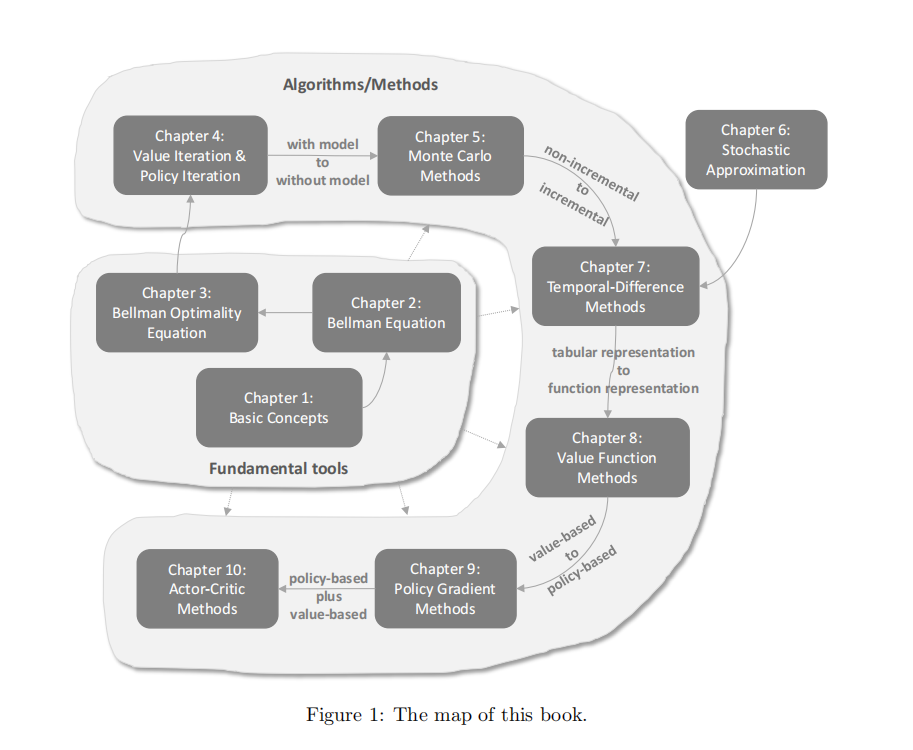
• Not just the map of this course, but also for RL fundations.
• Fundamental tools + Algorithms and methods.
• Importance of different parts.

1. Chapter 1: Basic Concepts
   • Concepts: state, action, reward, return, episode, policy,…
   • Grid-world examples
   • Markov decision process (MDP)
   • Fundamental concepts, widely used later
2. Chapter 2: Bellman Equations
   • One concept: state value

     $$\mathbb{v}_{\pi}(s) = \mathbb{E}[G_t | S_t = s]$$

   • One tool: Bellman equation

     $$\mathbb{v}_{\pi} = \mathbb{r}_{\pi} + \gamma P_{\pi} \mathbb{v}_{\pi}$$

   • Policy evaluation, widely used later
3. Chapter 3: Bellman Optimality Equations
   • A special Bellman equation
   • Two concepts: optimal policy $\pi^*$ and optimal state value $v^*(s)$
   • One tool: Bellman optimality equation

     $$\mathbb{v}^*(s) = \max_{\pi} (\mathbb{r}_{\pi} + \gamma P_{\pi} \mathbb{v}_{\pi}) = f(\mathbb{v})$$

     • Fixed-point theorem （不动点原理）
     • Fundamental problems
       • 最优策略、最优的 state value是否存在
       • 最优的 state value 是唯一的
       • 最优的策略可能是 deterministic，也可能是 stochastic
       • 一定存在确定性的最优策略
     • An algorithm solving the equation
   • Optimality, widely used later
4. Chapter 4: Value Iteration & Policy Iteration
   • First algorithms for optimal policies
   • Three algorithms:
     • Value iteration (VI) （值迭代）
     • Policy iteration (PI) （策略迭代）
     • Truncated policy iteration （截断策略迭代）
   • Policy update and value update, widely used later
   • Need the environment model
5. Chapter 5: Monte Carlo Learning
   • Gap: how to do model-free learning?
   • Mean estimation with sampling data

     $$E[X] \approx \overline{x} = \frac{1}{n} \sum_{i=1}^n X_i$$

   • First model-free RL algorithms
   • Algorithms:
     • MC Basic （基本的 MC 算法）
     • MC Exploring Starts （探索开始的 MC 算法）
     • MC $\epsilon$-greedy （基于 $\epsilon$-贪婪的 MC 算法）
6. Chapter 6: Stochastic Approximation
   • Gap: from non-incremental to incremental
   • Mean estimation
   • Algorithms:
     • Robbins-Monro (RM) algorithm （ Robbins-Monro 算法）
     • Stochastic gradient descent (SGD) （随机梯度下降算法）
     • SGD, BGD, MBGD
7. Chapter 7: Temporal-Difference Learning
   • Classic RL algorithms
   • Algorithms:
     • TD learning of state values （TD 学习状态值）
     • SARSA: TD learning of action values （TD 学习动作值）
     • Q-learning: TD learning of optimal action values （TD 学习最优动作值）
     • On-policy & off-policy （基于策略与非基于策略）
       • 强化学习中有两个策略：
         • behavior policy，用于生成经验数据
         • target policy，用于指导价值函数的更新
       • 如果 behavior policy 与 target policy 相同，即 $\pi = \mu$，则称为 on-policy learning（基于策略学习）
       • 如果 behavior policy 与 target policy 不同，即 $\pi \neq \mu$，则称为 off-policy learning（非基于策略学习）
     • Unified point of view
8. Chapter 8: Value Function Approximation
   • Gap: tabular representation to function representation
   • Algorithms:
     • State value estimation with value function approximation (VFA) （状态值估计与价值函数近似）:

       $$\min_{\pi} J(w) = \mathbb{E}[v_{\pi}(S) - \hat{v}(S,w)]$$

     • SARSA with VFA （Sarsa 算法与价值函数近似）
     • Q-learning with VFA （Q-learning 算法与价值函数近似）
     • Deep Q-learning
   • Neural networks come into RL
9. Chapter 9: Policy Gradient Methods
   • Gap: from value-based to policy-based
   • Contents:
     • Metrics to define optimal policies:

       $$J(\theta) = \overline{v}_{\pi}, \overline{r}_{\pi}$$

     • Policy gradient:

       $$\nabla J(\theta) = \mathbb{E}[\nabla_{\theta} \ln \pi(A | S) q_{\pi}(S, A)]$$

     • Gradient-ascent algorithm (REINFORCE):

       $$\theta_{t+1} = \theta_{t} + \alpha \nabla_{\theta} \ln \pi (a_t | s_t, \theta_t) q_t (s_t, a_t)$$

10. Chapter 10: Actor-Critic Methods
    • Gap: policy-based + value-based

      $$\theta_{t+1} = \theta_{t} + \alpha \nabla_{\theta} \ln \pi (a_t | s_t, \theta_t) q_t (s_t, a_t)$$

    • Algorithms:
      • The simplest actor-critic (QAC)
      • Advantage actor-critic (A2C)
        • 引入了一个 baseline $b(s_t)$，用于减少方差
      • Off-policy actor-critic
        • 使用 Importance sampling 的方法使得 QAC 由 on-policy 向 off-policy 转换
      • Deterministic actor-critic (DPG)

Lecture 1: Basic Concepts in Reinforcement Learning

Contents

• First, introduce fundamental concepts in RL by examples.
• Second, formalize the conceptts in the context of Markov decision process.

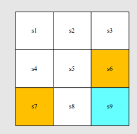
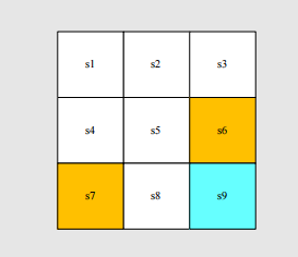
A grid-world example

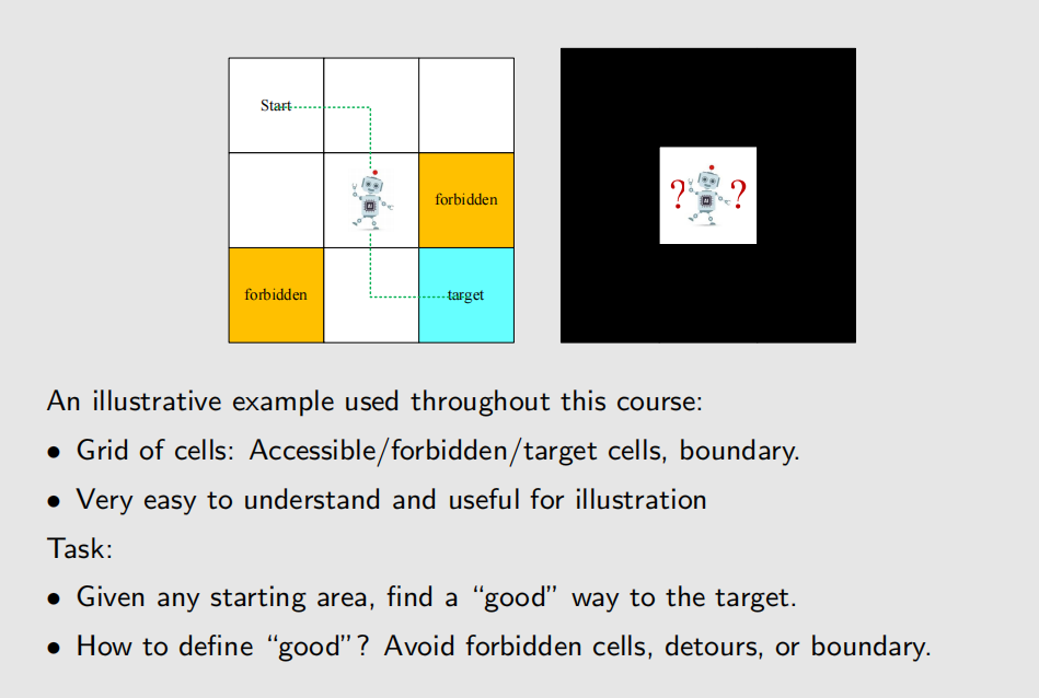
State

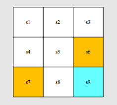
State: The status of the agent with respect to the environment

• 针对于 grid-world 示例，state 指的是 location，如下图中一共有 9 个 location，也就对应了 9 个 state。

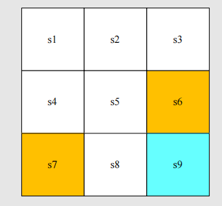
State space: The set of all states $\mathbb{S} = {s_i}^{9}_{i=1}$.

Action

Action: For each state, there are five possible actions: $a_1, \cdots, a_5$.

• $a_1$: move upwards
• $a_2$: move rightwards
• $a_3$: move downwards
• $a_4$: move leftwards
• $a_5$: stay in the same location

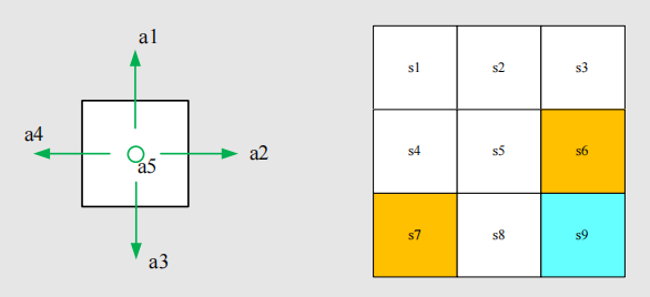
Action space: The set of all actions $\mathbb{A} = {a_i}^{5}_{i=1}$.

Question: Can different states have different sets of actions?

State transition

When taking an action, the agent may move from one state to another. Such a process is called state transition.

• At state $s_1$, if we choose action $a_2$, then what is the next state?

  $$s_1 \xrightarrow{a_2} s_2$$

• At state $s_1$, if we choose action $a_1$, then what is the next state?

  $$s_1 \xrightarrow{a_1} s_1$$

• State transition defines the interaction with the invironment.
• Question: Can we define the state transition in other ways?
  • Yes

Forbidden area: At state $s_5$, if we choose action $a_2$, then what is the next state?

• Case1: the forbidden area is accessible but with penalty. Then,

  $$s_5 \xrightarrow{a_2} s_6$$

• Case2: the forbiden area is inaccessible (e.g. surrounded by a wall).Then,

  $$s_5 \xrightarrow{a_2} s_5$$

We consider the first case, which is more general and challenging.

Tabular representation: We can use a table to describe the state transition:

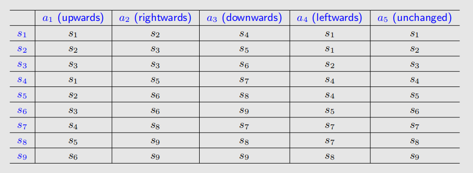
Can only represent deterministic cases.

State transition probability: Use probability to describe state transition!

• Intuition: At state $s_1$, if we choose action $a_2$, the next state is $s_2$.
• Math:
  $P(s_2 | s_1, a_2) = 1$
  $P(s_1 | s_1, a_2) = 0$

Here it is a deterministic case. The state transition could be stochastic (for example, wind gust).

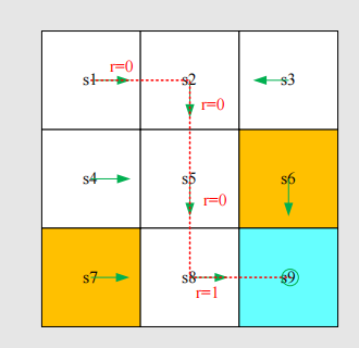
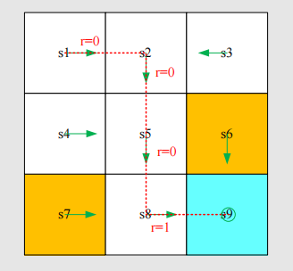
Policy

Policy tells the agent whay actions to take at a state.

Intuitive representation: The arrows demonstrate a policy.

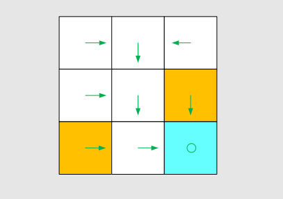
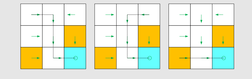
Based on this policy, we get the following paths with different starting points.

Mathmatical representation: using conditional probability
For example, for state $s_1$ :

$$\begin{aligned} \pi(a_1|s_1) &= 0 \\ \pi(a_2|s_1) &= 1 \\ \pi(a_3|s_1) &= 0 \\ \pi(a_4|s_1) &= 0 \\ \pi(a_5|s_1) &= 0 \\ \end{aligned}$$

It’s a deterministic policy.

There are stochastic policies.

For example:

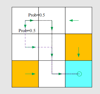
In this policy, for $s_1$:

$$\begin{aligned} \pi(a_1|s_1) &= 0 \\ \pi(a_2|s_1) &= 0.5 \\ \pi(a_3|s_1) &= 0.5 \\ \pi(a_4|s_1) &= 0 \\ \pi(a_5|s_1) &= 0 \\ \end{aligned}$$

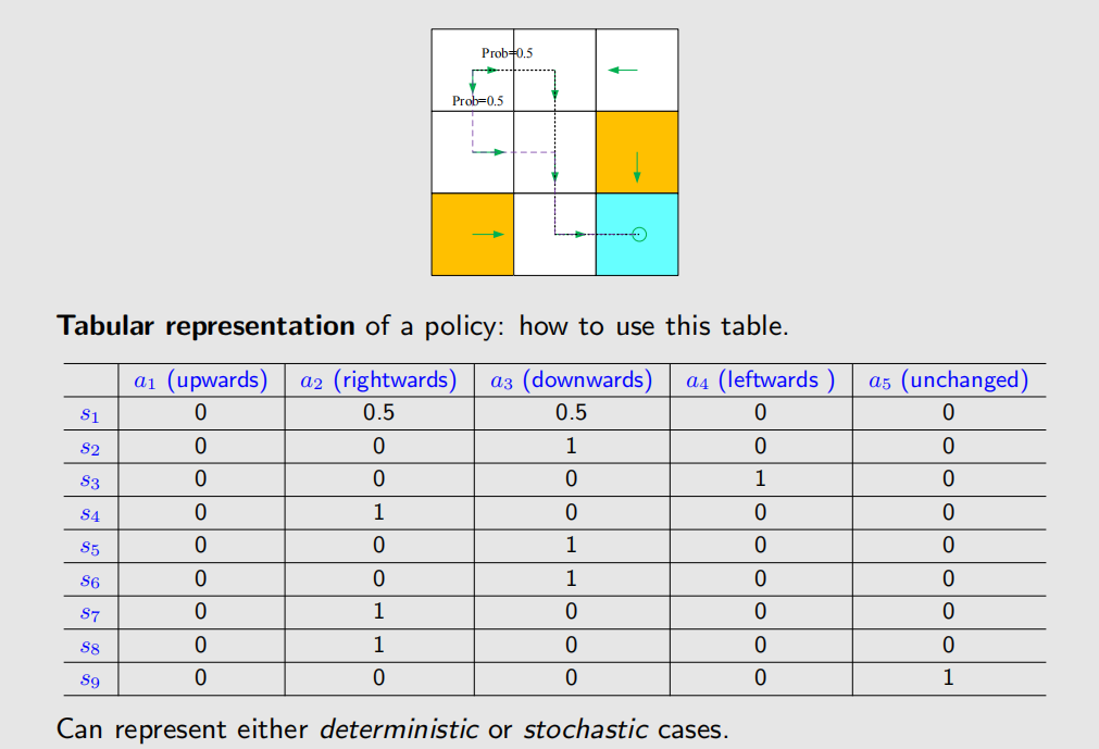
这种表格非常的 general，我们可以用它来描述任意的 policy。

在编程中如何实现概率表达呢，我们可以选取一个采样区间 [0,1]：

• if $x \in [0, 0.5)$, take action $a_1$;
• if $x \in [0.5, 1]$, take action $a_2$;

Reward

Reward is one of the most unique concepts of RL.

Reward: a real number we get after taking an action.

• A positive reward represents encouragement to take such actions.
• A negative reward represents punishment to take such actions.

Questins:

• What about a zero reward?
  • No punishment.
• Can positive mean punishment?
  • Yes.

In the grid-world example, the rewards are designed as follows:

• If the agent attemps to get out of boundary, let $r_{bound} = -1$
• If the agent attemps to enter a forbidden cell, let $r_{forbid} = -1$
• If the agent reches the target cell, let $r_{target} = +1$
• Otherwise, the agent gets a reward of $r = 0$.

Reward can be interpreted as a human-machine interface, with which we can guide the agent to behave as what we expect.

For example, with the above designed rewards, the agent will try to avoid getting out of the boundary or stepping into the forbidden cells.

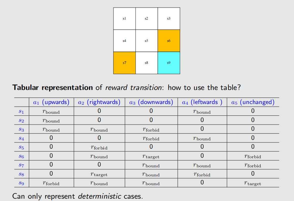
Mathematical description: conditional probability

• Intuition: At state $s_1$, if we choose action $a_1$, the reward is $-1$.
• Math: $p(r = -1|s_1, a_1) = 1$ and $p(r \neq -1|s_1, a_1) = 0$

Remarks:

• Here it is a deterministic case. The reward transition could be stochastic.
• For example, if you study hard, you will get rewards. But how much is uncertain.
• The reward depends on the state and action, but not the next state (for example, consider $s_1,a_1$ and $s_1,a_5$).

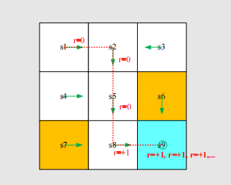
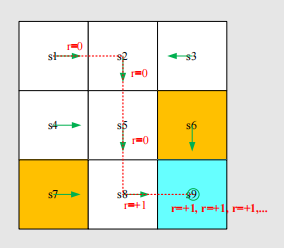
Trajectory and return

A trajectory is a state-action-reward chain:

$$S_1 \xrightarrow[{r=0}]{a_2} S_2 \xrightarrow[{r=0}]{a_3} S_5 \xrightarrow[{r=0}]{a_3} S_8 \xrightarrow[{r=1}]{a_2} S_9$$

The return of this trajectory is the sum of all the rewards collected along the trajectory:

$$return = 0 + 0 + 0 + 1 = 1$$

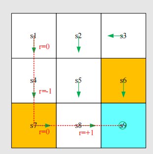
A different policy gives a different trajectory:

$$S_1 \xrightarrow[{r=0}]{a_3} S_4 \xrightarrow[{r=-1}]{a_3} S_7 \xrightarrow[{r=0}]{a_2} S_8 \xrightarrow[{r=+1}]{a_2} S_9$$

The return of this path is:

$$return = 0 + (-1) + 0 + 1 = 0$$

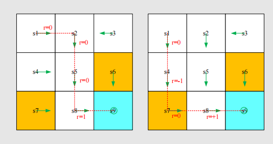
Which policy is better?

• Intuition: the first is better, because it avoids the forbidden areas.
• Mathematics: the first one is better, since it has a greater return!
• Return could be used to evaluate whether a policy is good or not (see details in the next lecture)!

Discounted return

A trajectory may be infinite:

$$S_1 \xrightarrow{a_2} S_2 \xrightarrow{a_3} S_5 \xrightarrow{a_3} S_8 \xrightarrow{a_2} S_9 \xrightarrow{\color{red}{a_5}} \color{red}{S_9} \xrightarrow{\color{red}{a_5}} \color{red}{S_9} \cdots$$

The return is

$$return = 0 + 0 + 0 + 1 + 1 + 1 + ... = \infty$$

The definition is invalid since the return diverges!

Need to introduce a discount rate $\gamma \in [0,1)$

Discounted return:

$$\begin{aligned} discounted\ return &= 0 + \gamma 0 + \gamma^2 0 +\gamma^3 1 + \gamma^4 1 + \gamma^5 + 1 + \cdots \\ &= \gamma^3 (1 + \gamma + \gamma^2 + \gamma^3 + \cdots) \\ &= \gamma^3 (\frac{1}{1 - \gamma}) \end{aligned}$$

Roles:

1. The sum becomes finite.
2. Balance the far and near future rewards.

Explanation:

• If $\gamma$ is close to 0, the value of the discounted return is dominated by the rewards obtained in the near future.
• If $\gamma$ is close to 1, the value of the discounted return is dominated by the rewards obtained in the far future.
• 简而言之，如果 $\gamma$ 比较小，那 discounted return 比较近视；如果 $\gamma$ 比较大，那 discounted return 比较远视。

Episode

强化学习（Reinforcement Learning）中，episode 是一个核心概念，指的是智能体（agent）与环境（environment）交互的完整序列，从初始状态开始，到终止状态（terminal state）结束，期间不会被打断。
序列构成：一个 episode 由 状态（state）→ 行动（action）→ 奖励（reward）→ 下一状态（next state） 的循环组成，直到触发终止条件（例如游戏结束、任务完成等）

When interacting with the environment following a policy, the agent may stop at some terminal state. The resulting trajectory is called an episode (or a trial).

Example: episode

$$S_1 \xrightarrow[{r=0}]{a_2} S_2 \xrightarrow[{r=0}]{a_3} S_5 \xrightarrow[{r=0}]{a_3} S_8 \xrightarrow[{r=1}]{a_2} S_9$$

An episode is usually assumed to be a finite trajectory. Tasks with episodes are called episodic tasks.

Some tasks may have no terminal states, meaning the interaction with the environment will never end. Such tasks are called continuing tasks.

In the grid-world example, should we stop after arriving the target?

In fact, we can treat episodic and continuing tasks in a unified mathematical way by converting episodic tasks to continuing tasks.

• Option 1: Treat the target state as a special absorbing state. Once the agent reaches an absorbing state, it will never leave. The consequent rewards $r = 0$.
• Option 2: Treat the target state as a normal state with a policy. The agent can still leave the target state and gain $r = +1$ when entering the target state.

We consider option 2 in this course so that we don’t need to distinguish the target state from the others and can treat it as a normal state.

Markov decision process (MDP)

Key elements of MDP:

• Sets:
  • State: the set of states $\mathbb{S}$.
  • Action: the set of actions $\mathbb{A}(s)$ is associated for state $s \in \mathbb{S}$.
  • Reward: the set of rewards $\mathbb{R}(s,a)$.
• Probability distribution:
  • State transition probability: at state $s$, taking action $a$, the probability to transit to state $s'$ is $p(s'|s,a)$
  • Reward probability: at state $s$, taking action $a$, the probability to get reward $r$ is $p(r|s,a)$
• Policy: at state $s$, the probability to choose action $a$ is $\pi(a|s)$
• Markov property: memoryless property

  $$p(s_{t+1}|a_t,s_t,\cdots,a_0,s_0) = p(s_{t+1}|a_t,s_t)$$

  $$p(r_{t+1}|a_t,s_t,\cdots,a_0,s_0) = p(r_{t+1}|a_t,s_t)$$

All the concepts introduced in this lecture can be put in the framework in MDP.

The grid world could be abstracted as a more general model, Markov process.

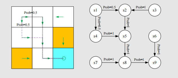
The circle represent states and the links with arrows represent the state transition.

Markov decision process becomes Markov process once the policy is given.

MDP VS MP

马尔科夫过程(Markov Process, MP)和马尔科夫决策过程(Markov Decision Process, MDP)是强化学习中的两个核心概念，它们之间存在重要的区别：

马尔科夫过程 (Markov Process, MP)

马尔科夫过程是一个二元组 $(S, P)$，其中：

• $S$ 是状态空间
• $P$ 是状态转移概率矩阵

特点：

• 被动性：系统状态的转移是自动发生的，没有外部决策者的干预
• 随机性：状态转移完全由概率决定
• 马尔科夫性：下一个状态只依赖于当前状态，与历史无关

数学表达：

$$P(S_{t+1} = s' | S_t = s, S_{t-1} = s_{t-1}, \ldots, S_0 = s_0) = P(S_{t+1} = s' | S_t = s)$$

马尔科夫决策过程 (Markov Decision Process, MDP)

马尔科夫决策过程是一个四元组 $(S, A, P, R)$，其中：

• $S$ 是状态空间
• $A$ 是动作空间
• $P$ 是状态转移概率矩阵（依赖于动作）
• $R$ 是奖励函数

特点：

• 主动性：存在决策者（智能体）可以选择动作
• 目标导向：通过奖励机制引导决策
• 策略依赖：状态转移依赖于所选择的动作

数学表达：

$$P(S_{t+1} = s' | S_t = s, A_t = a) = P_{ss'}^a$$

$$R(S_t = s, A_t = a, S_{t+1} = s') = R_{ss'}^a$$

主要区别对比

关系总结

• MP是MDP的特殊情况：当MDP中只有一个动作可选时，MDP退化为MP
• MDP扩展了MP：在MP基础上增加了动作选择和奖励机制
• 从描述到控制：MP描述系统行为，MDP控制系统行为

Summary

By using grid-world examples, we demonstrated the following key concepts:

• State
• Action
• State transition, state transition probability $p(s'|s,a)$
• Reward, reward probability $p(r|s,a)$
• Trajectory, episode, return, discounted return
• Markov decision process

Lecture 2: